z.test <- function(y, mu = 0, sigma = 1,
                   alternative = c('two.sided', 'less', 'greater'),
                   conf.level = 0.95) {

  alternative <- match.arg(alternative)
  message(paste('Number of missing values:', sum(is.na(y))))
  y_orig <- y
  y <- y[!is.na(y)]
  # Calculations here
  xbar <- mean(y)
  n <- length(y)
  se <- sigma / sqrt(n)
  z <- (xbar-mu)/se
  alpha <- 1-conf.level

  # Hypothesis tests
  if(alternative == "two.sided") {
    lcl <- xbar - qnorm(1-alpha/2)*se
    ucl <- xbar + qnorm(1-alpha/2)*se
    p.value <- 2*pnorm(abs(z), lower.tail = F)
  } else if (alternative == 'less') {
    lcl <- -Inf
    ucl <- xbar + qnorm(1-alpha)*se
    p.value <- pnorm(z)
  } else if (alternative == 'greater') {
    lcl <- xbar - qnorm(1-alpha)*se
    ucl <- Inf
    p.value <- pnorm(z, lower.tail = FALSE)
  } else {
    stop("Invalid alternative provided")
  }


  # Organize results
  results <- list(
    data = y_orig,                                      # Original data
    sample_mean = xbar,                                # Mean of the data
    standard_error = se,                             # Standard error
    z = z,                                          # Test statistic
    parameters = list(mu = mu, sigma = sigma),     # Parameters
    alternative = alternative,                     # The alternative hypothesis
    alpha = alpha,                                      # Significance level
    confidence_interval = list(lcl = lcl, ucl = ucl),    # Confidence interval
    p.value = p.value                                     # p-value of the test

  )

  # Output list of results
  return(results)
}Project 2 Solutions
Problem 1
Problem 2
Part a
z.test.data <- read.csv('z-test-data.csv')
z.test(y=z.test.data$prob2a,
       mu=30, sigma=sd(z.test.data$prob2a),
       alternative = 'greater')
Number of missing values: 0$data
[1] 31.3 28.8 31.0 29.8 28.8 33.6 29.5 35.6 29.8 37.4 34.1 36.3 34.9 36.4 32.7
[16] 34.2 33.8 29.4 31.7 28.2 26.5 30.0 35.3 32.1 32.5 30.7 34.4 32.3 30.3 32.6
[31] 29.5 32.8 38.9 31.1 31.1 24.2 26.5 30.8 29.1 31.5
$sample_mean
[1] 31.7375
$standard_error
[1] 0.4895404
$z
[1] 3.549247
$parameters
$parameters$mu
[1] 30
$parameters$sigma
[1] 3.096126
$alternative
[1] "greater"
$alpha
[1] 0.05
$confidence_interval
$confidence_interval$lcl
[1] 30.93228
$confidence_interval$ucl
[1] Inf
$p.value
[1] 0.0001931671The p-value is less than 0.05, meaning that we reject the null hypothesis. There is evidence to conclude that the true mean is greater than 30.
Part b
z.test(y=z.test.data$prob2b,
       mu=15, sigma=sd(z.test.data$prob2b),
       alternative = 'less')
Number of missing values: 0$data
[1] 19.8 18.4 7.6 14.3 15.8 10.7 13.0 11.1 10.2 18.5 14.4 13.6 5.6 15.4 19.4
[16] 17.9 12.4 21.8 18.8 23.1 8.8 22.8 8.5 8.0 20.1 15.9 14.5 21.6 20.3 14.5
[31] 15.0 12.0 12.0 14.5 13.0 14.6 8.6 8.0 21.1 5.5
$sample_mean
[1] 14.5275
$standard_error
[1] 0.7744062
$z
[1] -0.6101449
$parameters
$parameters$mu
[1] 15
$parameters$sigma
[1] 4.897775
$alternative
[1] "less"
$alpha
[1] 0.05
$confidence_interval
$confidence_interval$lcl
[1] -Inf
$confidence_interval$ucl
[1] 15.80128
$p.value
[1] 0.2708829The p-value is greater than 0.05, meaning that we fail to reject the null hypothesis. There is not evidence to conclude that the true mean is less than 15.
Part c
z.test(y=z.test.data$prob2c,
       mu=50, sigma=sd(z.test.data$prob2c),
       alternative = 'two.sided')
Number of missing values: 0$data
[1] 55.9 55.5 55.2 61.7 46.5 59.9 53.9 52.5 54.0 53.4 54.9 55.5 59.4 55.8 56.7
[16] 48.1 52.0 54.3 61.2 54.2 49.7 57.5 60.1 51.5 50.1 53.2 52.7 54.7 60.7 48.3
[31] 51.1 51.3 55.4 59.0 59.3 54.0 54.8 52.2 46.9 52.0
$sample_mean
[1] 54.3775
$standard_error
[1] 0.6132876
$z
[1] 7.137761
$parameters
$parameters$mu
[1] 50
$parameters$sigma
[1] 3.878771
$alternative
[1] "two.sided"
$alpha
[1] 0.05
$confidence_interval
$confidence_interval$lcl
[1] 53.17548
$confidence_interval$ucl
[1] 55.57952
$p.value
[1] 9.486344e-13The p-value is less than 0.05, meaning that we reject the null hypothesis. There is evidence to conclude that the true mean is different from 50.
Problem 3
mn_river <- read.csv('mn-river-n-samples.csv')
y <- mn_river$N_mg_l
qqnorm(y); qqline(y)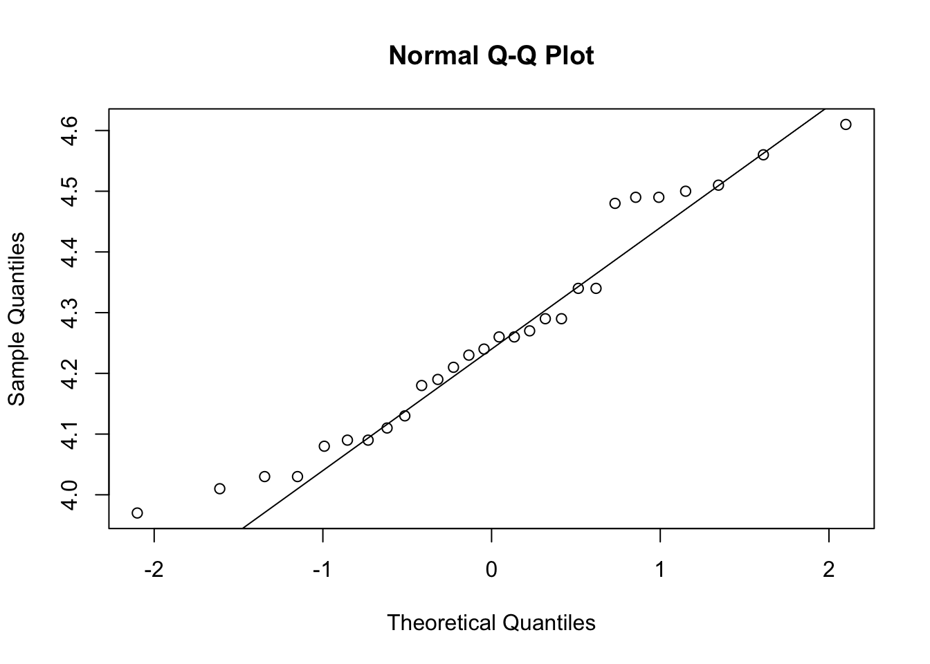
hist(y)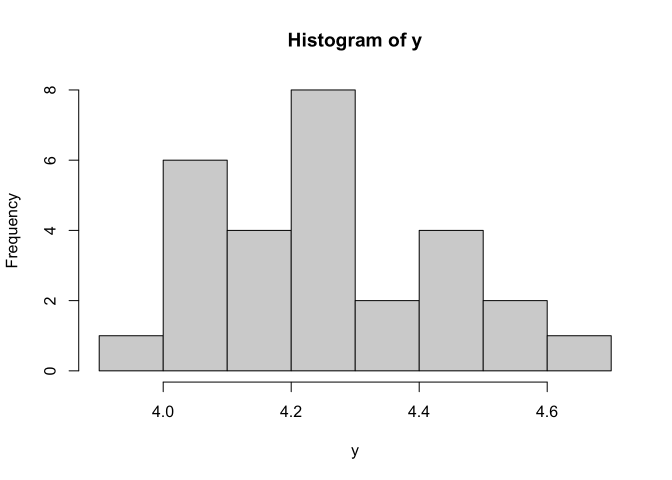
boxplot(y)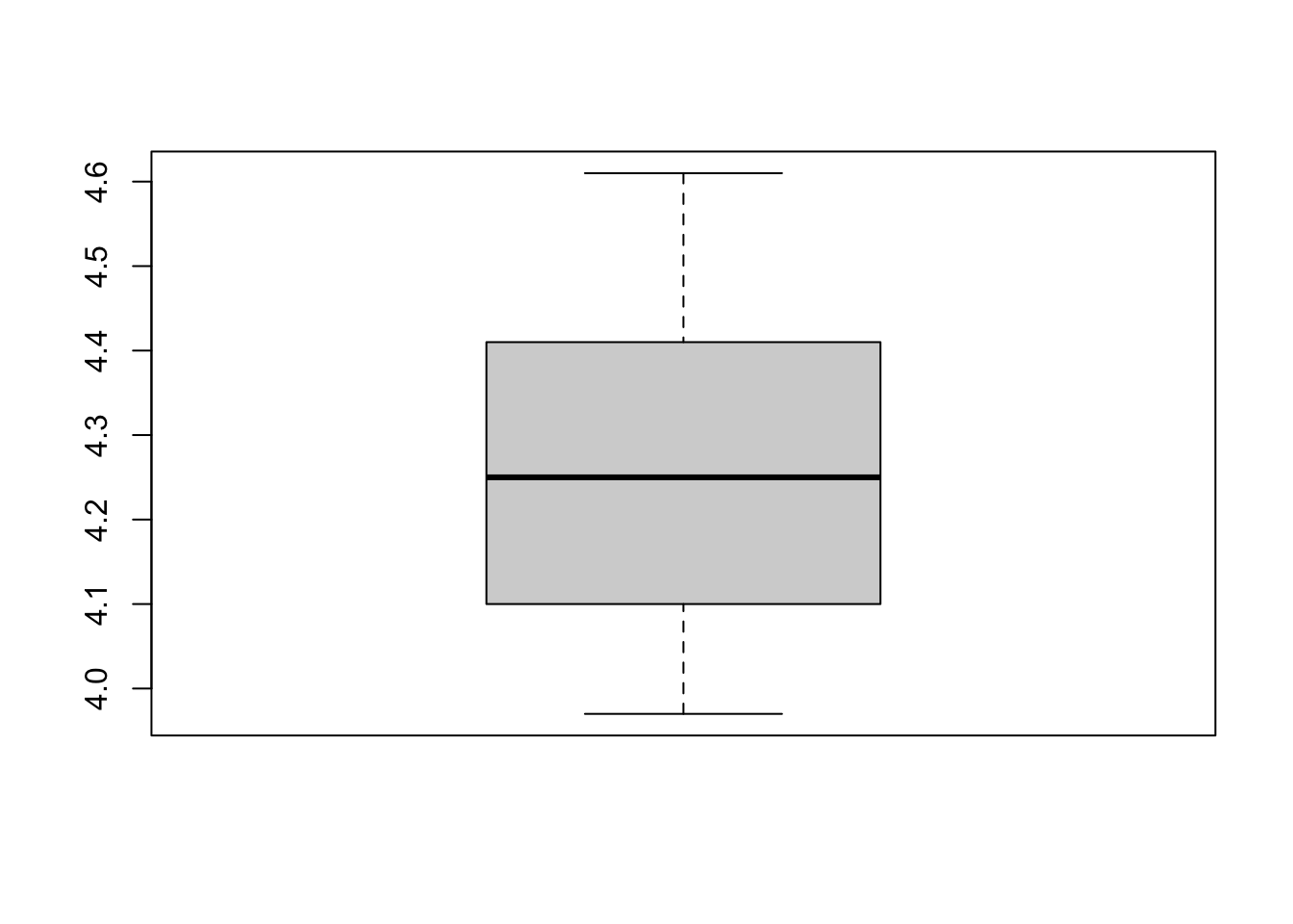
For the part, values tend to follow the line in the Q-Q plot. The histogram shows a little bit of skewness, but nothing out of the ordinary. The boxplot looks fairly symmetrical. The data appears to be approximately normally distributed.
Problem 4
\[ H_0: \mu=4.19 \]
\[ H_0: \mu>4.19 \]
Problem 5
# Remove missing values
y <- y[!is.na(y)]

# Calculate necessary values
n <- length(y)
xbar <- mean(y)
alpha <- 0.05
se <- sd(y)/sqrt(n)

test_statistic <- (xbar-4.19)/se
p_value <- pt(test_statistic, df = n-1, lower.tail = F)
ci <- xbar + c(-1,1)*qt(p=1-alpha, df=n-1)*se
knitr::kable(data.frame(
  test_statistic = test_statistic,
  p_value = p_value,
  lower_cl = ci[1],
  upper_cl = Inf
))| test_statistic | p_value | lower_cl | upper_cl |
|---|---|---|---|
| 2.030372 | 0.0261377 | 4.201277 | Inf |
Problem 6
t.test(x=y, alternative = 'greater', mu = 4.19)
    One Sample t-test

data:  y
t = 2.0304, df = 27, p-value = 0.02614
alternative hypothesis: true mean is greater than 4.19
95 percent confidence interval:
 4.201277      Inf
sample estimates:
mean of x
     4.26
Problem 7
The results of (5) and (6) are the same, but (6) is in a more structured format.
Problem 8
There is evidence to conclude that the true average Nitrogen (in mg/L) in the Minnesota River is greater than the previous historical average of 0.19 (p-value=0.02614). With 95% confidence, the true average quantity of Nitrogen is greater than 4.201 mg/L.