Problem 1
Read in the data and print the first 10 observations.
ne_work_commute <- read.csv("travel-time-31109.csv")
head(ne_work_commute, n=10)
   RESPONDENT TRANTIME DEPARTS ARRIVES
1           1        7     647     654
2           2        8    1305    1309
3           3       10    1445    1454
4           4       10    1605    1614
5           5       10    1605    1614
6           6       15    1515    1534
7           7       15    1435    1449
8           8        7    1545    1554
9           9       12    1535    1544
10         10       15    1435    1449
Problem 2
Use dim() to determine the dimensions of the dataset.
The dataset contains 861 rows and 4 columns.
Problem 3
Compute the mean of TRANTIME.
mean(ne_work_commute$TRANTIME)
The mean travel time is 18.35 minutes.
Problem 4
Compute the median of TRANTIME.
median(ne_work_commute$TRANTIME)
The median travel time is 15 minutes.
Problem 5
Compute the variance of TRANTIME.
var(ne_work_commute$TRANTIME)
The variance of travel time is 193.33 minutes squared.
Variance measures the amount of variability in travel time using squared deviations from the mean.
Problem 6
Compute the standard deviation of TRANTIME.
sd(ne_work_commute$TRANTIME)
The standard deviation of travel time is 13.9 minutes.
Problem 7
Use summary() on TRANTIME.
summary(ne_work_commute$TRANTIME)
   Min. 1st Qu.  Median    Mean 3rd Qu.    Max.
   1.00   10.00   15.00   18.35   20.00  129.00
The values returned by summary() have the following interpretations:
- Minimum: The smallest observed travel time.
- 1st Quartile: The value below which approximately 25% of observations fall.
- Median: The middle travel time.
- Mean: The arithmetic average travel time.
- 3rd Quartile: The value below which approximately 75% of observations fall.
- Maximum: The largest observed travel time.
Problem 8
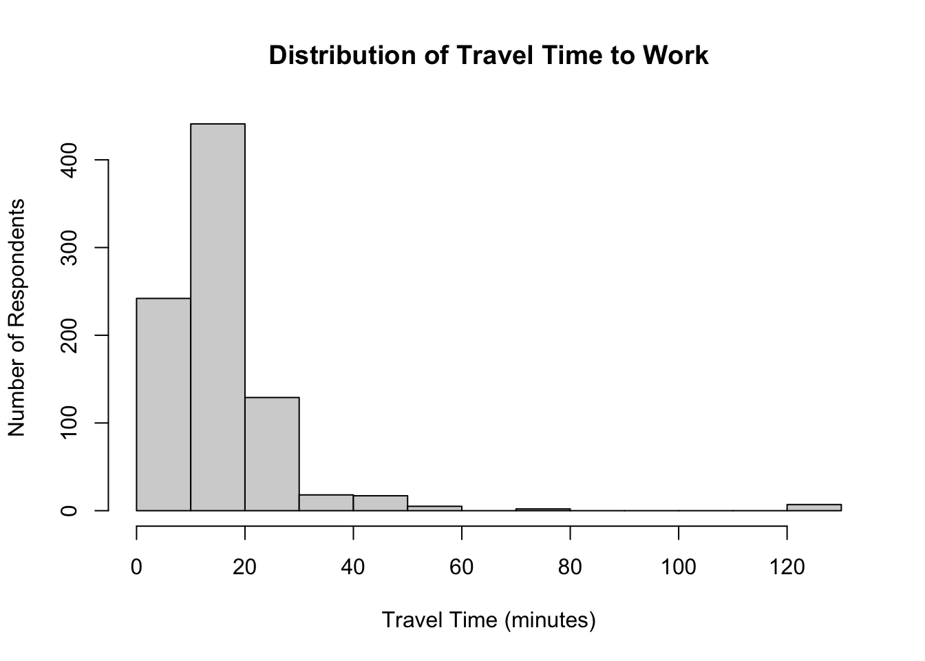
Create a histogram of TRANTIME.
hist(
  ne_work_commute$TRANTIME,
  main = "Distribution of Travel Time to Work",
  xlab = "Travel Time (minutes)",
  ylab = "Number of Respondents"
)
The data is right-skewed with large outliers.
Problem 9
Would the mean or median be a better description of travel time?
The median would be a better description since there are large values that would increase the mean.
Problem 10
Create filtered_travel_time by removing outliers using the IQR method.
An observation is considered an outlier if
\[
x < Q_1 - 1.5(IQR)
\]
or
\[
x > Q_3 + 1.5(IQR).
\]
First calculate the quartiles and IQR.
ne_summary <- summary(ne_work_commute$TRANTIME)

iqr <- IQR(ne_work_commute$TRANTIME)

q1 <- as.numeric(ne_summary[2])
q3 <- as.numeric(ne_summary[5])
iqr
Calculate the lower and upper boundaries:
lower_bound <- q1 - 1.5 * iqr
upper_bound <- q3 + 1.5 * iqr

lower_bound
Now retain only observations within these boundaries:
filtered_travel_time <- ne_work_commute$TRANTIME[
  ne_work_commute$TRANTIME >= lower_bound &
  ne_work_commute$TRANTIME <= upper_bound
]
Problem 11
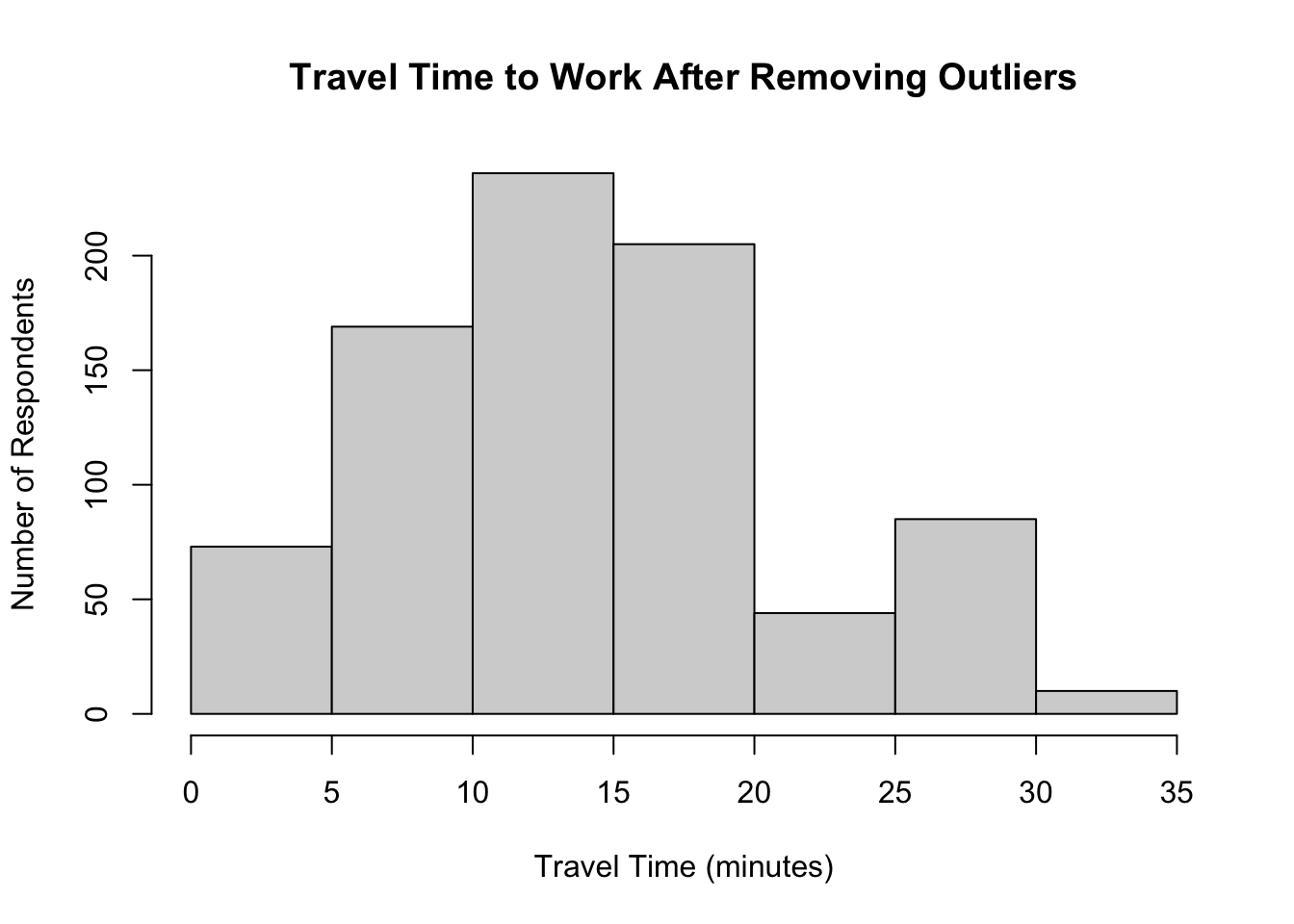
Create a histogram of filtered_travel_time.
hist(
  filtered_travel_time,
  main = "Travel Time to Work After Removing Outliers",
  xlab = "Travel Time (minutes)",
  ylab = "Number of Respondents"
)
After removing the outliers, the data is somewhat symmetrical with some right-skew.
Problem 12
Repeat Problems 3–6 using filtered_travel_time and arrange the results into a formatted table.
filtered_summary <- data.frame(
  Statistic = c(
    "Mean",
    "Median",
    "Variance",
    "Standard Deviation"
  ),
  Value = c(
    mean(filtered_travel_time),
    median(filtered_travel_time),
    var(filtered_travel_time),
    sd(filtered_travel_time)
  )
)

knitr::kable(
  filtered_summary,
  digits = 2,
  col.names = c("Statistic", "Value"),
  caption = "Summary Statistics After Removing Outliers"
)
Summary Statistics After Removing Outliers
| Mean |
16.24 |
| Median |
15.00 |
| Variance |
54.74 |
| Standard Deviation |
7.40 |
Problem 13
Describe what changed after removing the outliers.
Calculate the original and filtered summary statistics:
original_stats <- c(
  Mean = mean(ne_work_commute$TRANTIME),
  Median = median(ne_work_commute$TRANTIME),
  Variance = var(ne_work_commute$TRANTIME),
  SD = sd(ne_work_commute$TRANTIME)
)

filtered_stats <- c(
  Mean = mean(filtered_travel_time),
  Median = median(filtered_travel_time),
  Variance = var(filtered_travel_time),
  SD = sd(filtered_travel_time)
)

rbind(
  Original = original_stats,
  Filtered = filtered_stats
)
             Mean Median  Variance        SD
Original 18.34727     15 193.32926 13.904289
Filtered 16.23601     15  54.74082  7.398704
The median stayed the same. The mean slightly decreased, and the variance / standard deviation greatly decreased.
Problem 14
Let \(X\) be normally distributed with the mean and variance calculated from filtered_travel_time.
Thus,
\[
X \sim N(\mu,\sigma^2),
\]
where \(\mu\) and \(\sigma^2\) are the mean and variance of filtered_travel_time.
mu <- mean(filtered_travel_time)
sigma <- sd(filtered_travel_time)

mu
Note that pnorm() requires the standard deviation, not the variance, so sigma is supplied to the sd argument.
(a) Probability of less than 10 minutes
p_less_10 <- pnorm(
  10,
  mean = mu,
  sd = sigma
)

p_less_10
(b) Probability of between 10 and 20 minutes
We want
\[
P(10 < X < 20).
\]
Using cumulative probabilities,
\[
P(10 < X < 20)
=
P(X < 20)-P(X < 10).
\]
p_10_20 <- pnorm(
  20,
  mean = mu,
  sd = sigma
) -
  pnorm(
    10,
    mean = mu,
    sd = sigma
  )

p_10_20
(c) Probability of greater than 20 minutes
We want
\[
P(X > 20).
\]
Using the complement,
\[
P(X > 20)=1-P(X\leq20).
\]
p_greater_20 <- 1 - pnorm(
  20,
  mean = mu,
  sd = sigma
)

p_greater_20