Two-way ANOVA
Two-way ANOVA
What is ANOVA?
- ANalysis Of VAriance
- Compare the means of three or more treatment groups
- Extension of the t-test
When to use two-way ANOVA?
- Analyze the effect of two independent variables on a single response
- Effect of fertilizer type and planting density when measuring crop yield
- Effect of sugar and flour when measuring cake consistency
Two-way ANOVA
Model
Let A and B represent two factors. A has levels \(i=1\dots a\) and B has levels \(j=1\dots b\), and there are \(k=1\dots r\) replications. The model is given by:
\[ Y_{ijk}=\mu + A_i+B_j+(AB)_{ij}+\epsilon_{ijk} \]
Where
- \(Y_{ijk}\) is the response for the \(k\)th replication of level \(i\) for factor A and level \(j\) for factor B.
- \(\mu\) is the overall mean
- \(A_i\) is the effect of level \(i\) for factor A
- \(B_j\) is the effect of level \(j\) for factor B
- \((AB)_{ij}\) is the interaction effect
- \(\epsilon_{ijk}\sim iid \quad Normal(0, \sigma^2)\)
Model, cont.
Assumptions
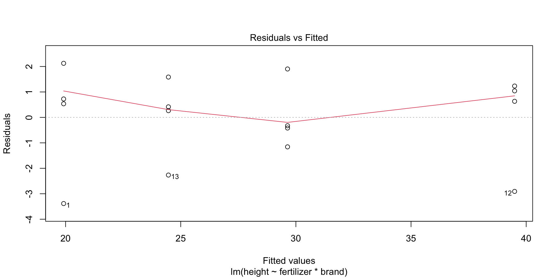
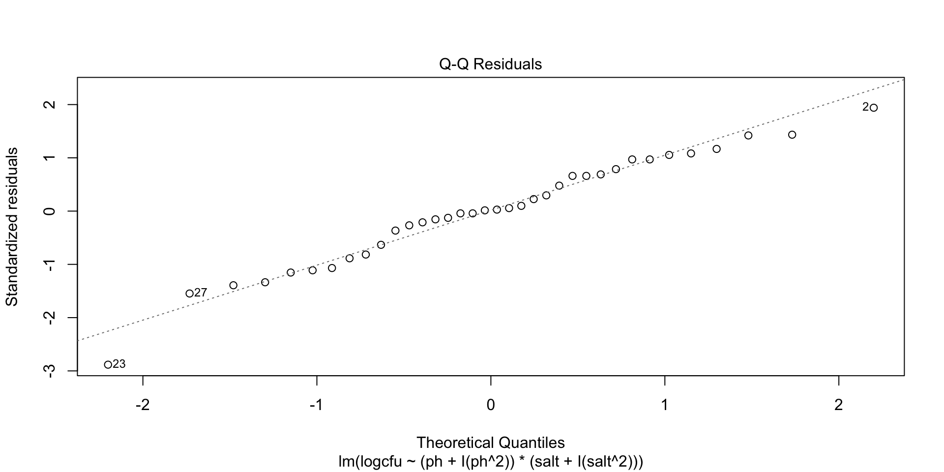
- Residuals are normally distributed
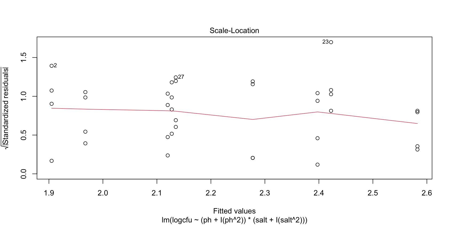
- Homogeneity of variance (variance is constant)
- Independence of observations
ANOVA Table
| Source | Sum of Squares | df | Mean Square | |
|---|---|---|---|---|
| Factor A | \(rb\sum_{i=1}^a(\bar{Y}_{i\cdot\cdot}-\bar{Y}_{\cdot\cdot\cdot})^2\) | \(a-1\) | \(MS_A=\frac{SS_A}{(a-1)}\) | |
| Factor B | \(ra\sum_{j=1}^b(\bar{Y}_{\cdot j\cdot}-\bar{Y}_{\cdot\cdot\cdot})^2\) | \(b-1\) | \(MS_B=\frac{SS_B}{(b-1)}\) | |
| Interaction (A x B) | \(r\sum_{i=1}^a\sum_{j=1}^b(\bar{Y}_{ij\cdot}-\bar{Y}_{i\cdot\cdot}-\bar{Y}_{\cdot j\cdot}+\bar{Y}_{\cdot\cdot\cdot})^2\) | \((a-1)(b-1)\) | \(MS_{AB}=\frac{SS_{AB}}{(a-1)(b-1)}\) | |
| Error | \(\sum_{i=1}^a\sum_{j=1}^b\sum_{k=1}^r(Y_{ijk}-\bar{Y}_{ij\cdot})^2\) | \(ab(r-1)\) | \(MS_E=\frac{SS_E}{ab(r-1)}\) | |
| Total | \(\sum_{i=1}^a\sum_{j=1}^b\sum_{k=1}^r(Y_{ijk}-\bar{Y}_{\cdot\cdot\cdot})^2\) | \(abr-1\) |
p-values are calculated by taking the probability of observing the F-statistic or larger values from an F-distribution.
To compute the F-statistic, take the mean square for the term of interest and divide by MSE. Under \(H_0\), this will follow an F-distribution with numerator degrees of freedom for the term of interest and denominator degrees of freedom for the error term.
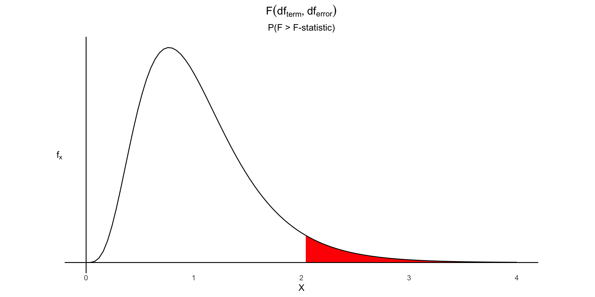
Calculation of p-value under an F distribution.
Example 1: Fertilizer Experiment
Example 1
An experiment was conducted to measure the effect of fertilizer on the growth height of a plant. Researchers used two brands of fertilizers (Easy-Plant and Fast-Grow) with two quantities (low and high). Each combination of fertilizer brand and quantity were applied to individual pots of plants, measuring the plant height after a set growing period.
Interaction plots
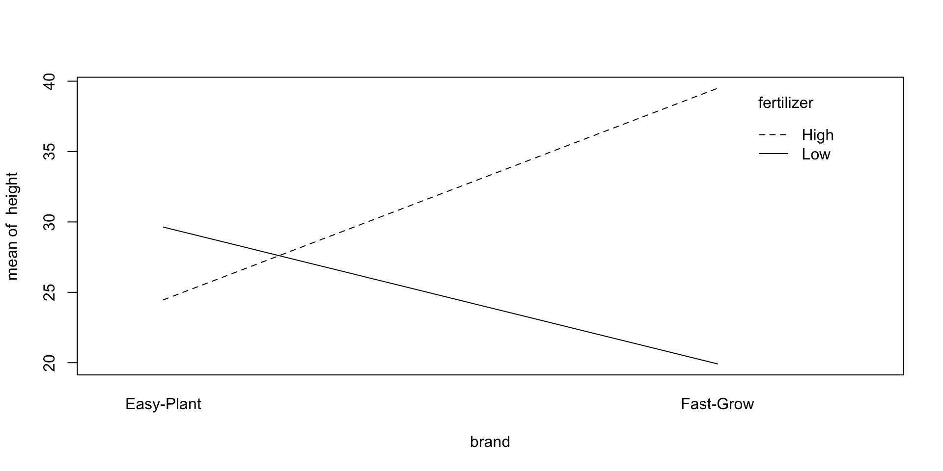
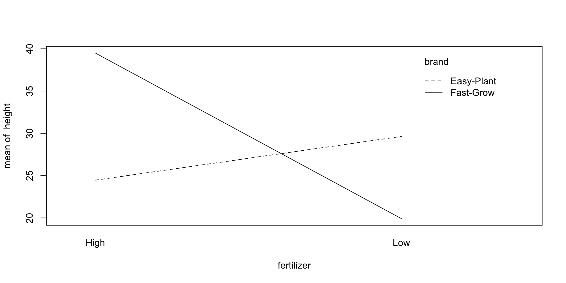
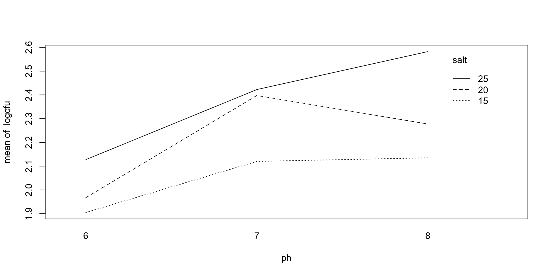
The interaction term of our model is not always required. To visualize whether this term is needed, we can create interaction plots. These are created by plotting the mean of each treatment combination against one treatment variable, and distinguishing the other treatment variable in the plot.
- If the lines are parallel, then there is not likely an interaction.
Interaction plots, cont.
Fitting a model
Call:
lm(formula = height ~ fertilizer * brand, data = agriculture)

Coefficients:
                 (Intercept)                 fertilizerLow
                      24.465                         5.173
              brandFast-Grow  fertilizerLow:brandFast-Grow
15.033 -24.755 Model Summary
Call:
lm(formula = height ~ fertilizer * brand, data = agriculture)

Residuals:
    Min      1Q  Median      3Q     Max
-3.3850 -0.6025  0.4750  1.0900  2.1250

Coefficients:
                             Estimate Std. Error t value Pr(>|t|)
(Intercept)                   24.4650     0.9284   26.35 5.46e-12 ***
fertilizerLow                  5.1725     1.3129    3.94  0.00196 **
brandFast-Grow                15.0325     1.3129   11.45 8.15e-08 ***
fertilizerLow:brandFast-Grow -24.7550     1.8568  -13.33 1.48e-08 ***
---
Signif. codes:  0 '***' 0.001 '**' 0.01 '*' 0.05 '.' 0.1 ' ' 1

Residual standard error: 1.857 on 12 degrees of freedom
Multiple R-squared:  0.9535,    Adjusted R-squared:  0.9419
F-statistic: 82.05 on 3 and 12 DF,  p-value: 2.899e-08
ANOVA Table
Analysis of Variance Table

Response: height
                 Df Sum Sq Mean Sq  F value    Pr(>F)
fertilizer        1 207.65  207.65  60.2301 5.123e-06 ***
brand             1  28.20   28.20   8.1785   0.01436 *
fertilizer:brand  1 612.81  612.81 177.7508 1.484e-08 ***
Residuals        12  41.37    3.45
---
Signif. codes: 0 '***' 0.001 '**' 0.01 '*' 0.05 '.' 0.1 ' ' 1Anova Table (Type III tests)
Response: height
Sum Sq Df F value Pr(>F)
(Intercept) 2394.14 1 694.442 5.459e-12 ***
fertilizer 53.51 1 15.521 0.001964 **
brand 451.95 1 131.093 8.145e-08 ***
fertilizer:brand 612.81 1 177.751 1.484e-08 ***
Residuals 41.37 12
---
Signif. codes: 0 '***' 0.001 '**' 0.01 '*' 0.05 '.' 0.1 ' ' 1Estimated Means
The interaction term was significant, so we should only consider differences at each treatment combination.
 brand      fertilizer emmean    SE df lower.CL upper.CL
 Easy-Plant High         24.5 0.928 12     22.4     26.5
 Fast-Grow  High         39.5 0.928 12     37.5     41.5
 Easy-Plant Low          29.6 0.928 12     27.6     31.7
 Fast-Grow  Low          19.9 0.928 12     17.9     21.9

Confidence level used: 0.95 brand = Easy-Plant:
fertilizer emmean SE df lower.CL upper.CL
High 24.5 0.928 12 22.4 26.5
Low 29.6 0.928 12 27.6 31.7
brand = Fast-Grow:
fertilizer emmean SE df lower.CL upper.CL
High 39.5 0.928 12 37.5 41.5
Low 19.9 0.928 12 17.9 21.9
Confidence level used: 0.95 Estimated differences
 contrast                             estimate   SE df t.ratio p.value
 (Easy-Plant High) - (Fast-Grow High)   -15.03 1.31 12 -11.450 <0.0001
 (Easy-Plant High) - (Easy-Plant Low)    -5.17 1.31 12  -3.940  0.0092
 (Easy-Plant High) - (Fast-Grow Low)      4.55 1.31 12   3.466  0.0210
 (Fast-Grow High) - (Easy-Plant Low)      9.86 1.31 12   7.510 <0.0001
 (Fast-Grow High) - (Fast-Grow Low)      19.58 1.31 12  14.915 <0.0001
 (Easy-Plant Low) - (Fast-Grow Low)       9.72 1.31 12   7.405 <0.0001

P value adjustment: tukey method for comparing a family of 4 estimates contrast estimate SE df lower.CL upper.CL
(Easy-Plant High) - (Fast-Grow High) -15.03 1.31 12 -18.930 -11.13
(Easy-Plant High) - (Easy-Plant Low) -5.17 1.31 12 -9.070 -1.27
(Easy-Plant High) - (Fast-Grow Low) 4.55 1.31 12 0.652 8.45
(Fast-Grow High) - (Easy-Plant Low) 9.86 1.31 12 5.962 13.76
(Fast-Grow High) - (Fast-Grow Low) 19.58 1.31 12 15.685 23.48
(Easy-Plant Low) - (Fast-Grow Low) 9.72 1.31 12 5.825 13.62
t.ratio p.value
-11.450 <0.0001
-3.940 0.0092
3.466 0.0210
7.510 <0.0001
14.915 <0.0001
7.405 <0.0001
Confidence level used: 0.95
Conf-level adjustment: tukey method for comparing a family of 4 estimates
P value adjustment: tukey method for comparing a family of 4 estimates Fit of model
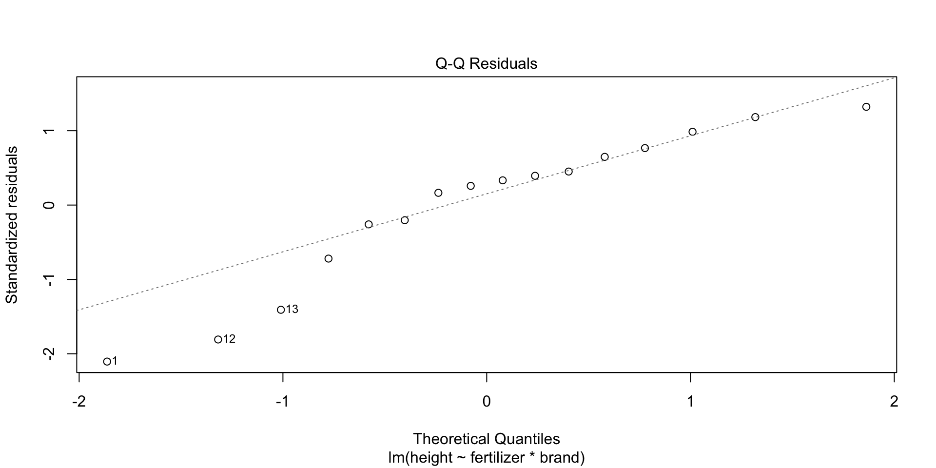
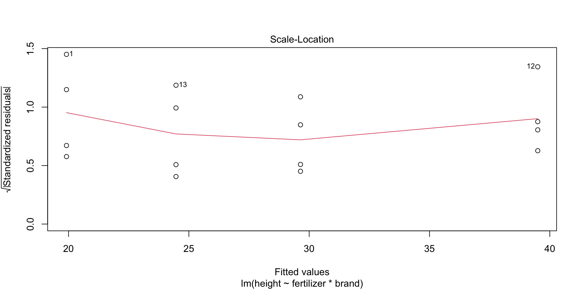
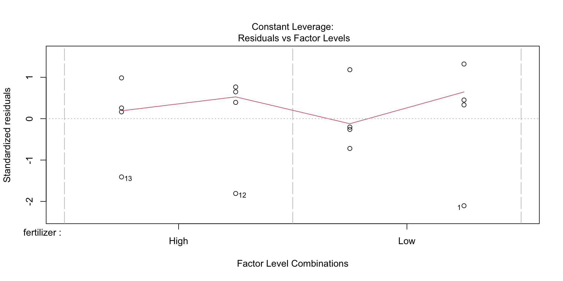
Example 2: Bacteria Growth
Example 2
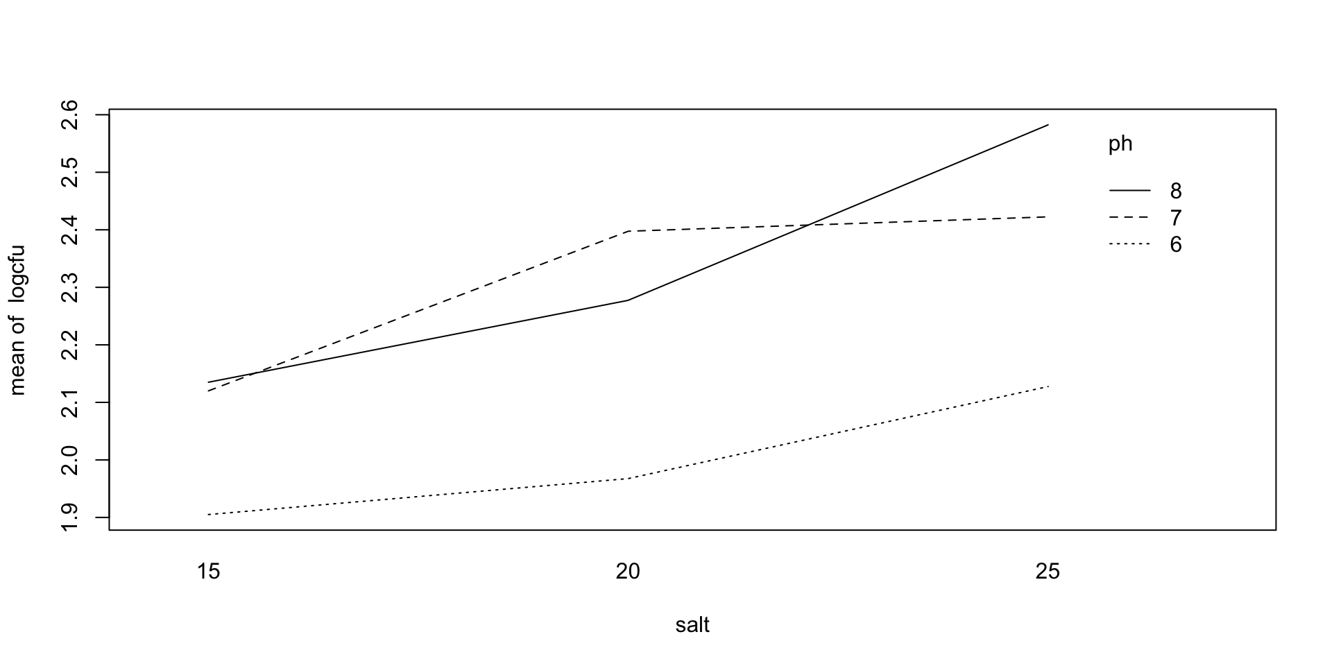
An experiment was conducted to measure the effect of pH and salt concentration on bacteria growth. Bacteria were placed into Petri dishes and were given a solution that consisted of a pH and salt concentration combination. pH levels were set at levels of 6, 7, and 8, and salt concentration levels were set at 15%, 20%, and 25%. After a set amount of time, the bacteria growth was measured by log CFU (colony forming unit).
Interaction plots
Fitting a model
Option 1: categorical factors
- Use this option if you are interested in the categories themselves.
- Same approach as previous example, but convert treatments to factors.
Option 2: quantitative factors
- Use this option if you are interested in measuring polynomial trends and/or making predictions.
Note: You can get the same results from both models using polynomial orthogonal contrasts.
Model Summary
Call:
lm(formula = logcfu ~ (ph + I(ph^2)) * (salt + I(salt^2)), data = bacteria)

Residuals:
     Min       1Q   Median       3Q      Max
-0.51250 -0.12062  0.00375  0.12688  0.34500

Coefficients:
                    Estimate Std. Error t value Pr(>|t|)
(Intercept)       131.722500 115.843558   1.137    0.265
ph                -37.890000  33.464837  -1.132    0.267
I(ph^2)             2.720000   2.388315   1.139    0.265
salt              -14.499250  11.978762  -1.210    0.237
I(salt^2)           0.365250   0.298692   1.223    0.232
ph:salt             4.223750   3.460420   1.221    0.233
ph:I(salt^2)       -0.106450   0.086286  -1.234    0.228
I(ph^2):salt       -0.302750   0.246963  -1.226    0.231
I(ph^2):I(salt^2)   0.007650   0.006158   1.242    0.225

Residual standard error: 0.2053 on 27 degrees of freedom
Multiple R-squared:  0.5819,    Adjusted R-squared:  0.458
F-statistic: 4.696 on 8 and 27 DF,  p-value: 0.001094
ANOVA Table
Analysis of Variance Table

Response: logcfu
                  Df  Sum Sq Mean Sq F value    Pr(>F)
ph                 1 0.66002 0.66002 15.6643 0.0004948 ***
I(ph^2)            1 0.17405 0.17405  4.1308 0.0520539 .
salt               1 0.63050 0.63050 14.9638 0.0006264 ***
I(salt^2)          1 0.00001 0.00001  0.0003 0.9863846
ph:salt            1 0.05062 0.05062  1.2015 0.2827051
ph:I(salt^2)       1 0.00141 0.00141  0.0334 0.8563030
I(ph^2):salt       1 0.00141 0.00141  0.0334 0.8563030
I(ph^2):I(salt^2)  1 0.06503 0.06503  1.5432 0.2248173
Residuals         27 1.13765 0.04214
---
Signif. codes:  0 '***' 0.001 '**' 0.01 '*' 0.05 '.' 0.1 ' ' 1
Estimated Means
 ph salt emmean    SE df lower.CL upper.CL
  7   20    2.4 0.103 27     2.19     2.61

Confidence level used: 0.95
What happened here??
Estimated Means
 ph salt emmean    SE df lower.CL upper.CL
  6   15   1.91 0.103 27     1.69     2.12
  7   15   2.12 0.103 27     1.91     2.33
  8   15   2.13 0.103 27     1.92     2.35
  6   20   1.97 0.103 27     1.76     2.18
  7   20   2.40 0.103 27     2.19     2.61
  8   20   2.28 0.103 27     2.07     2.49
  6   25   2.13 0.103 27     1.92     2.34
  7   25   2.42 0.103 27     2.21     2.63
  8   25   2.58 0.103 27     2.37     2.79

Confidence level used: 0.95
Differences
 contrast                estimate    SE df t.ratio p.value
 ph6 salt15 - ph7 salt15  -0.2150 0.145 27  -1.481  0.8544
 ph6 salt15 - ph8 salt15  -0.2300 0.145 27  -1.585  0.8046
 ph6 salt15 - ph6 salt20  -0.0625 0.145 27  -0.431  1.0000
 ph6 salt15 - ph7 salt20  -0.4925 0.145 27  -3.393  0.0469
 ph6 salt15 - ph8 salt20  -0.3725 0.145 27  -2.566  0.2464
 ph6 salt15 - ph6 salt25  -0.2225 0.145 27  -1.533  0.8304
 ph6 salt15 - ph7 salt25  -0.5175 0.145 27  -3.565  0.0317
 ph6 salt15 - ph8 salt25  -0.6775 0.145 27  -4.668  0.0021
 ph7 salt15 - ph8 salt15  -0.0150 0.145 27  -0.103  1.0000
 ph7 salt15 - ph6 salt20   0.1525 0.145 27   1.051  0.9766
 ph7 salt15 - ph7 salt20  -0.2775 0.145 27  -1.912  0.6120
 ph7 salt15 - ph8 salt20  -0.1575 0.145 27  -1.085  0.9716
 ph7 salt15 - ph6 salt25  -0.0075 0.145 27  -0.052  1.0000
 ph7 salt15 - ph7 salt25  -0.3025 0.145 27  -2.084  0.5035
 ph7 salt15 - ph8 salt25  -0.4625 0.145 27  -3.186  0.0739
 ph8 salt15 - ph6 salt20   0.1675 0.145 27   1.154  0.9595
 ph8 salt15 - ph7 salt20  -0.2625 0.145 27  -1.809  0.6765
 ph8 salt15 - ph8 salt20  -0.1425 0.145 27  -0.982  0.9845
 ph8 salt15 - ph6 salt25   0.0075 0.145 27   0.052  1.0000
 ph8 salt15 - ph7 salt25  -0.2875 0.145 27  -1.981  0.5684
 ph8 salt15 - ph8 salt25  -0.4475 0.145 27  -3.083  0.0919
 ph6 salt20 - ph7 salt20  -0.4300 0.145 27  -2.963  0.1176
 ph6 salt20 - ph8 salt20  -0.3100 0.145 27  -2.136  0.4718
 ph6 salt20 - ph6 salt25  -0.1600 0.145 27  -1.102  0.9689
 ph6 salt20 - ph7 salt25  -0.4550 0.145 27  -3.135  0.0824
 ph6 salt20 - ph8 salt25  -0.6150 0.145 27  -4.237  0.0062
 ph7 salt20 - ph8 salt20   0.1200 0.145 27   0.827  0.9949
 ph7 salt20 - ph6 salt25   0.2700 0.145 27   1.860  0.6445
 ph7 salt20 - ph7 salt25  -0.0250 0.145 27  -0.172  1.0000
 ph7 salt20 - ph8 salt25  -0.1850 0.145 27  -1.275  0.9303
 ph8 salt20 - ph6 salt25   0.1500 0.145 27   1.033  0.9788
 ph8 salt20 - ph7 salt25  -0.1450 0.145 27  -0.999  0.9828
 ph8 salt20 - ph8 salt25  -0.3050 0.145 27  -2.101  0.4929
 ph6 salt25 - ph7 salt25  -0.2950 0.145 27  -2.032  0.5358
 ph6 salt25 - ph8 salt25  -0.4550 0.145 27  -3.135  0.0824
 ph7 salt25 - ph8 salt25  -0.1600 0.145 27  -1.102  0.9689

P value adjustment: tukey method for comparing a family of 9 estimates
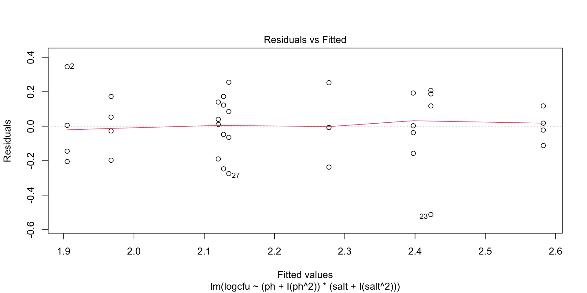
Fit of Model

Sums of Squares
- R uses Type I Sums of Squares by default.
- Type I: sequential fit, good for regression
- Type III: fits all together, good for categorical treatment factors
- For balanced design, these will give same result
STAT 801A