Randomized Complete Block Designs
Randomized Complete Block Design
What is a randomized complete block design (RCBD)?
- An experimental design that accounts for variability among experimental units.
- Experimental units are grouped into blocks based on a known source of variability.
- Every block receives every treatment exactly once.
- Treatments are randomized within each block.
Why use blocking?
- Reduce unexplained variability.
- Improve precision when comparing treatment means.
- Account for known sources of variability that are not the primary interest of the experiment.
Randomized Complete Block Design
Example:
Suppose we want to compare four fertilizers.
- We have four different fields with varying soil conditions.
- Each of three fields receives all four fertilizers.
- Within each field, the fertilizers are randomly assigned to experimental plots.
- Crop yield is measured for each plot.
The fields are our blocks, and fertilizer is our treatment.
Experimental Design
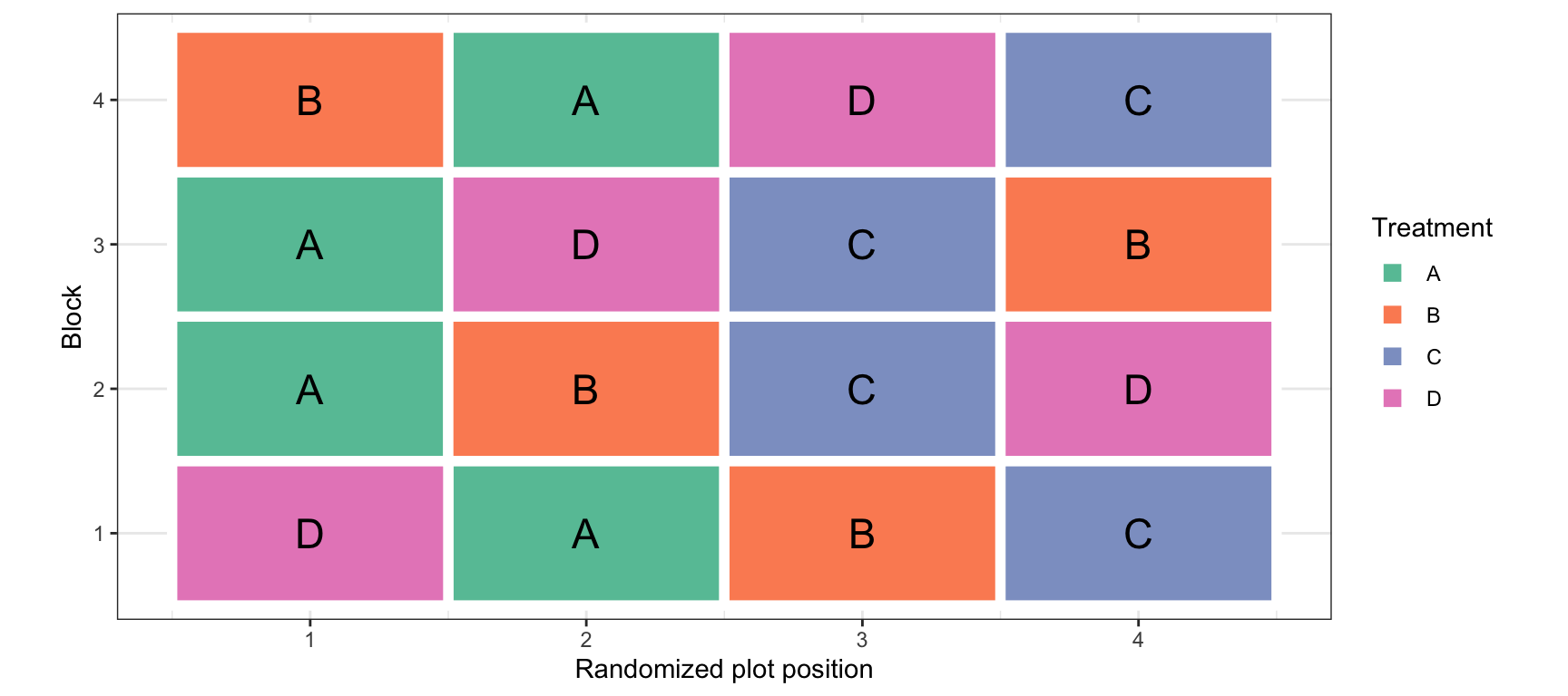
- Every block contains all four treatments.
- The order of treatments is randomized independently within each block.
Model
Let there be \(i=1,\ldots,a\) treatments and \(j=1,\ldots,b\) blocks.
The model is given by:
\[ Y_{ij}=\mu+\tau_i+\beta_j+\epsilon_{ij} \]
Where
- \(Y_{ij}\) is the response for treatment \(i\) in block \(j\).
- \(\mu\) is the overall mean.
- \(\tau_i\) is the effect of treatment \(i\).
- \(\beta_j\) is the effect of block \(j\).
- \(\epsilon_{ij}\sim iid\ Normal(0,\sigma^2)\).
Model, cont.
Assumptions
- Residuals are normally distributed.
- Homogeneity of variance (variance is constant).
- Independence of observations.
- No treatment-by-block interaction.
Why no interaction?
- Each treatment is observed only once in each block.
- There is no replication within treatment-block combinations.
- Therefore, treatment-by-block interaction cannot be separated from experimental error.
The model assumes that treatment differences are consistent across blocks.
Hypothesis Testing
Our primary interest is typically the treatment effect.
Treatment hypotheses:
\[ H_0:\tau_1=\tau_2=\cdots=\tau_a=0 \]
\[ H_A:\text{At least one }\tau_i\ne 0 \]
We may also test whether block effects are significant:
\[ H_0:\beta_1=\beta_2=\cdots=\beta_b=0 \]
\[ H_A:\text{At least one }\beta_j\ne 0 \]
However, blocks are generally included to account for variability rather than to make conclusions about the blocks themselves.
ANOVA Table
| Source | Sum of Squares | df | Mean Square |
|---|---|---|---|
| Treatment | \(b\sum_{i=1}^a(\bar Y_{i\cdot}-\bar Y_{\cdot\cdot})^2\) | \(a-1\) | \(SS_T/(a-1)\) |
| Block | \(a\sum_{j=1}^b(\bar Y_{\cdot j}-\bar Y_{\cdot\cdot})^2\) | \(b-1\) | \(SS_B/(b-1)\) |
| Error | \(SS_{Total}-SS_T-SS_B\) | \((a-1)(b-1)\) | \(SS_E/[(a-1)(b-1)]\) |
| Total | \(\sum_{i=1}^a\sum_{j=1}^b(Y_{ij}-\bar Y_{\cdot\cdot})^2\) | \(ab-1\) |
ANOVA Table, cont.
The treatment F-statistic is:
\[ F_T=\frac{MS_T}{MS_E} \]
Under the null hypothesis:
\[ F_T\sim F_{a-1,(a-1)(b-1)} \]
Similarly, the block F-statistic is:
\[ F_B=\frac{MS_B}{MS_E} \]
Sums of Squares
The total variation is partitioned into three components:
\[ SS_{Total}=SS_T+SS_B+SS_E \]
Treatment:
\[ SS_T=b\sum_{i=1}^a (\bar Y_{i\cdot}-\bar Y_{\cdot\cdot})^2 \]
Block:
\[ SS_B=a\sum_{j=1}^b (\bar Y_{\cdot j}-\bar Y_{\cdot\cdot})^2 \]
Error:
\[ SS_E=\sum_{i=1}^a\sum_{j=1}^b (Y_{ij}-\bar Y_{i\cdot}-\bar Y_{\cdot j} +\bar Y_{\cdot\cdot})^2 \]
Degrees of Freedom
The total degrees of freedom are:
\[ df_{Total}=ab-1 \]
The treatment degrees of freedom are:
\[ df_T=a-1 \]
The block degrees of freedom are:
\[ df_B=b-1 \]
The error degrees of freedom are:
\[ \begin{aligned} df_E&=(ab-1)-(a-1)-(b-1)\\ &=(a-1)(b-1) \end{aligned} \]
Example 1: Fertilizer Experiment
A researcher wants to compare four fertilizers to determine whether they differ in their effects on crop yield.
- Five fields are selected for the experiment.
- Each field is divided into four plots.
- Each fertilizer is randomly assigned to one plot within each field.
- Crop yield is measured for each plot.
Identify the experimental design.
- Treatment: Fertilizer
- Block: Field
- Response: Crop yield
Visualizing the Data
We can visualize the treatment and block effects using an interaction plot.
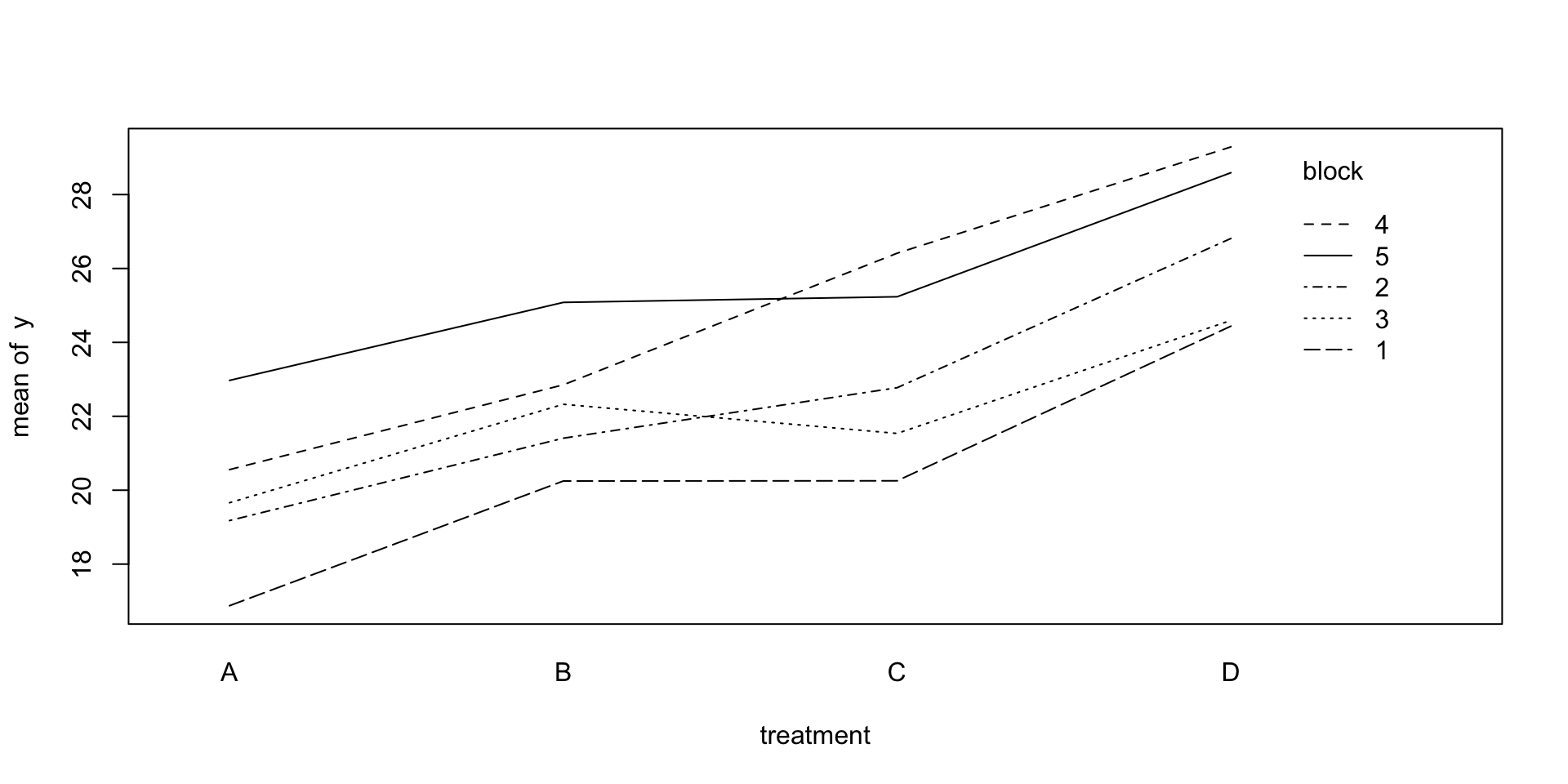
What do you notice?
- Are there differences among the treatments?
- Are there differences among the blocks?
- Do the treatment effects appear consistent across blocks?
Remember, the RCBD model assumes no treatment-by-block interaction.
Fitting a Model
We can fit the RCBD model using lm() or aov().
Call:
lm(formula = y ~ treatment + block, data = dat)

Residuals:
     Min       1Q   Median       3Q      Max
-2.15084 -0.52426  0.04488  0.58469  1.94399

Coefficients:
            Estimate Std. Error t value Pr(>|t|)
(Intercept)  16.1683     0.7205  22.441 5.91e-13 ***
treatmentB    2.5347     0.6990   3.626  0.00249 **
treatmentC    3.3940     0.6990   4.856  0.00021 ***
treatmentD    6.8973     0.6990   9.868 5.95e-08 ***
block         1.2266     0.1747   7.020 4.14e-06 ***
---
Signif. codes:  0 '***' 0.001 '**' 0.01 '*' 0.05 '.' 0.1 ' ' 1

Residual standard error: 1.105 on 15 degrees of freedom
Multiple R-squared:  0.9086,    Adjusted R-squared:  0.8842
F-statistic: 37.28 on 4 and 15 DF,  p-value: 1.259e-07
Fitting a Model, cont.
Notice that we use + rather than *.
treatment + block: Additive model.treatment * block: Includes an interaction term.
We cannot independently estimate the interaction and experimental error with only one observation per treatment-block combination.
ANOVA Table
Analysis of Variance Table

Response: y
          Df  Sum Sq Mean Sq F value    Pr(>F)
treatment  3 121.949  40.650  33.281 7.147e-07 ***
block      1  60.184  60.184  49.274 4.143e-06 ***
Residuals 15  18.321   1.221
---
Signif. codes:  0 '***' 0.001 '**' 0.01 '*' 0.05 '.' 0.1 ' ' 1
The ANOVA table provides tests for both treatment and block effects.
- Our primary interest is typically the treatment effect.
- The block effect accounts for differences among experimental units.
Estimated Means
We can use emmeans to obtain the estimated treatment means.
 treatment emmean    SE df lower.CL upper.CL
 A           19.8 0.494 15     18.8     20.9
 B           22.4 0.494 15     21.3     23.4
 C           23.2 0.494 15     22.2     24.3
 D           26.7 0.494 15     25.7     27.8

Confidence level used: 0.95
Because this is an additive model, the estimated treatment means account for differences among blocks.
Estimated Differences
We can use these comparisons to determine which fertilizer treatments differ from one another.
 contrast estimate    SE df lower.CL upper.CL t.ratio p.value
 A - B      -2.535 0.699 15    -4.55    -0.52  -3.626  0.0119
 A - C      -3.394 0.699 15    -5.41    -1.38  -4.856  0.0011
 A - D      -6.897 0.699 15    -8.91    -4.88  -9.868 <0.0001
 B - C      -0.859 0.699 15    -2.87     1.16  -1.229  0.6187
 B - D      -4.363 0.699 15    -6.38    -2.35  -6.241 <0.0001
 C - D      -3.503 0.699 15    -5.52    -1.49  -5.012  0.0008

Confidence level used: 0.95
Conf-level adjustment: tukey method for comparing a family of 4 estimates
P value adjustment: tukey method for comparing a family of 4 estimates
Fit of Model
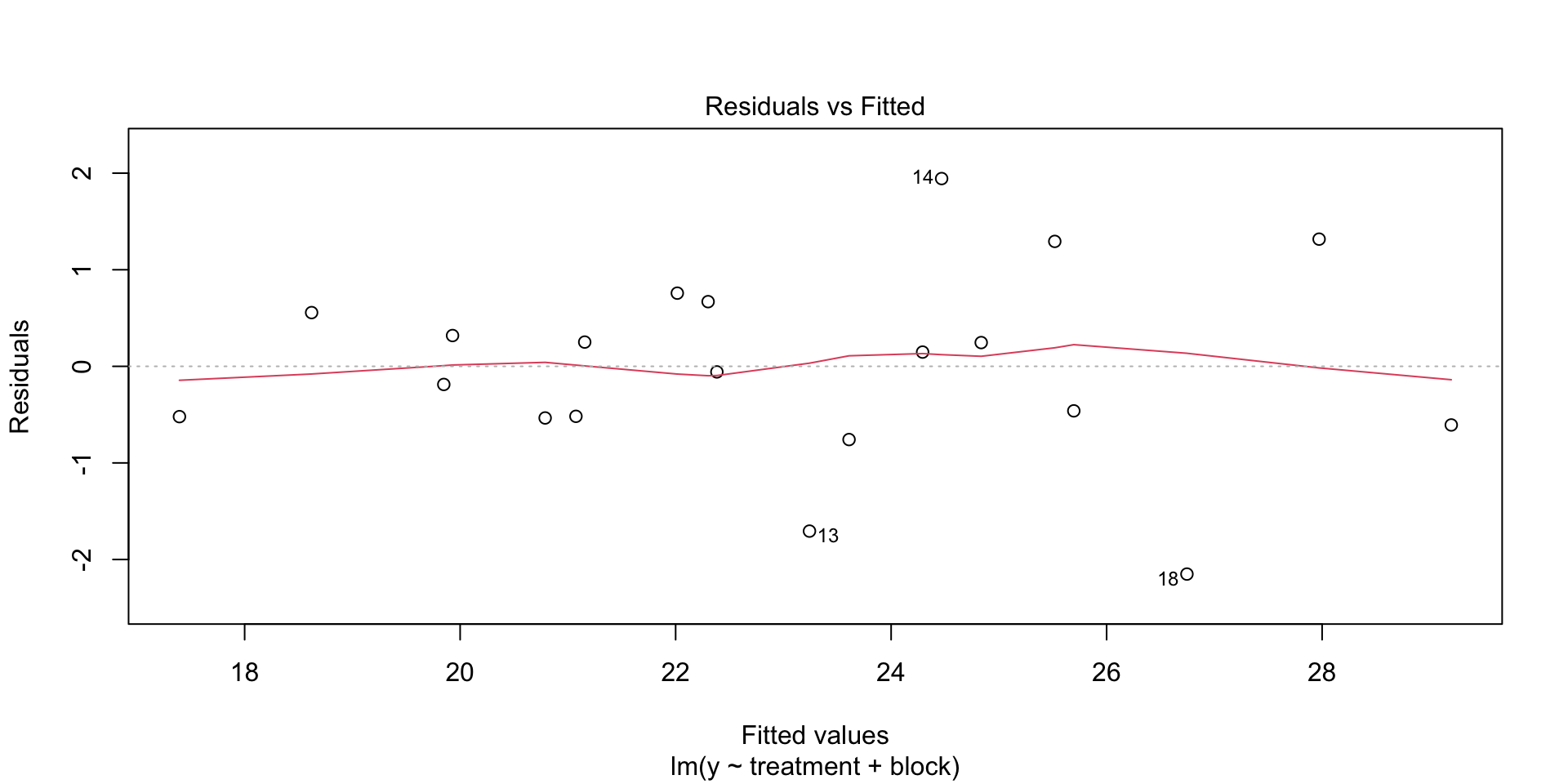
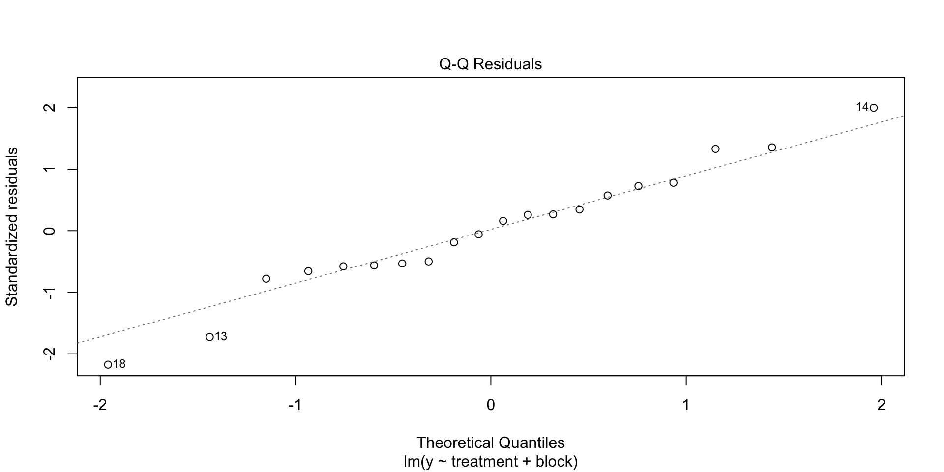
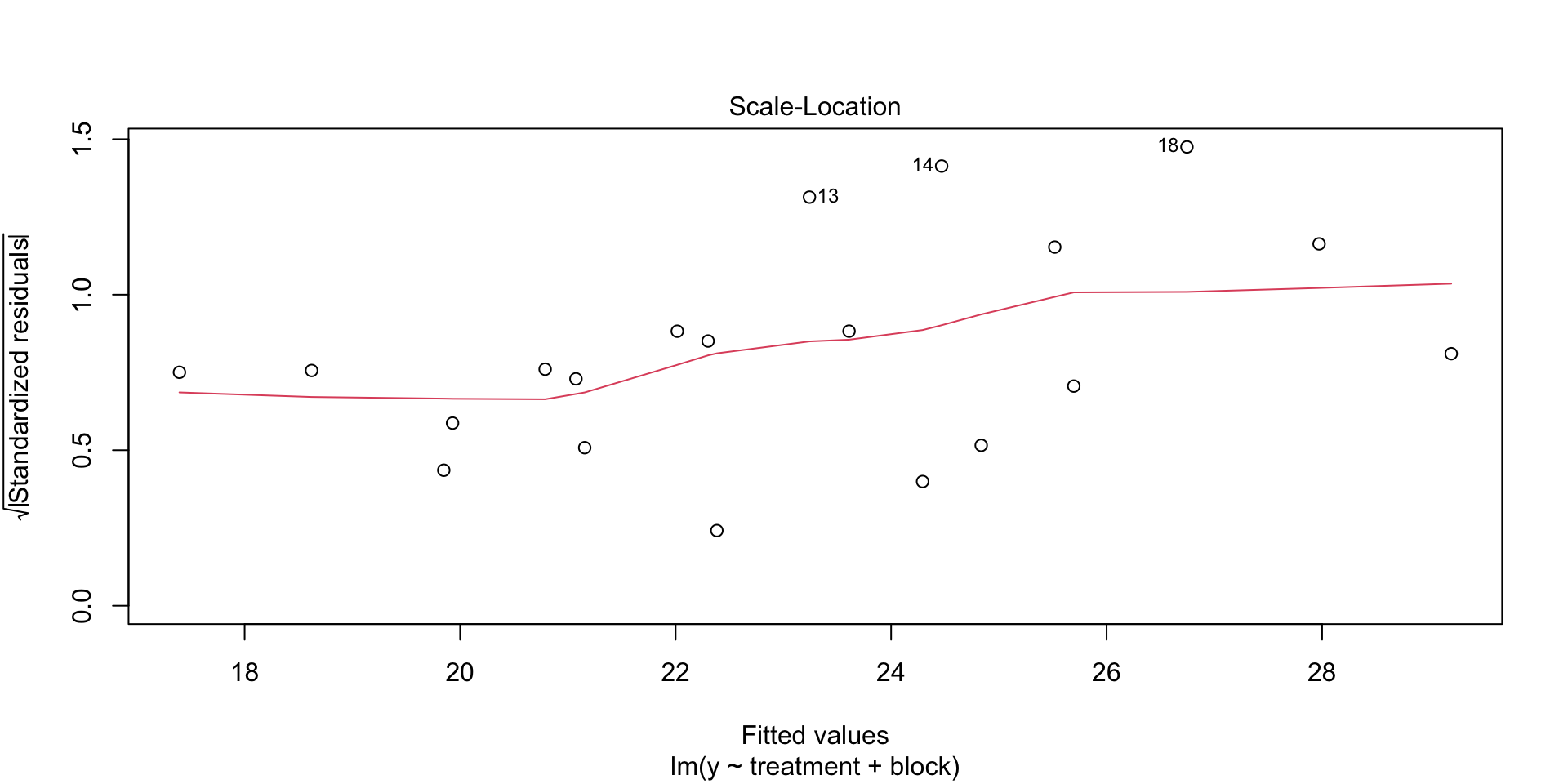
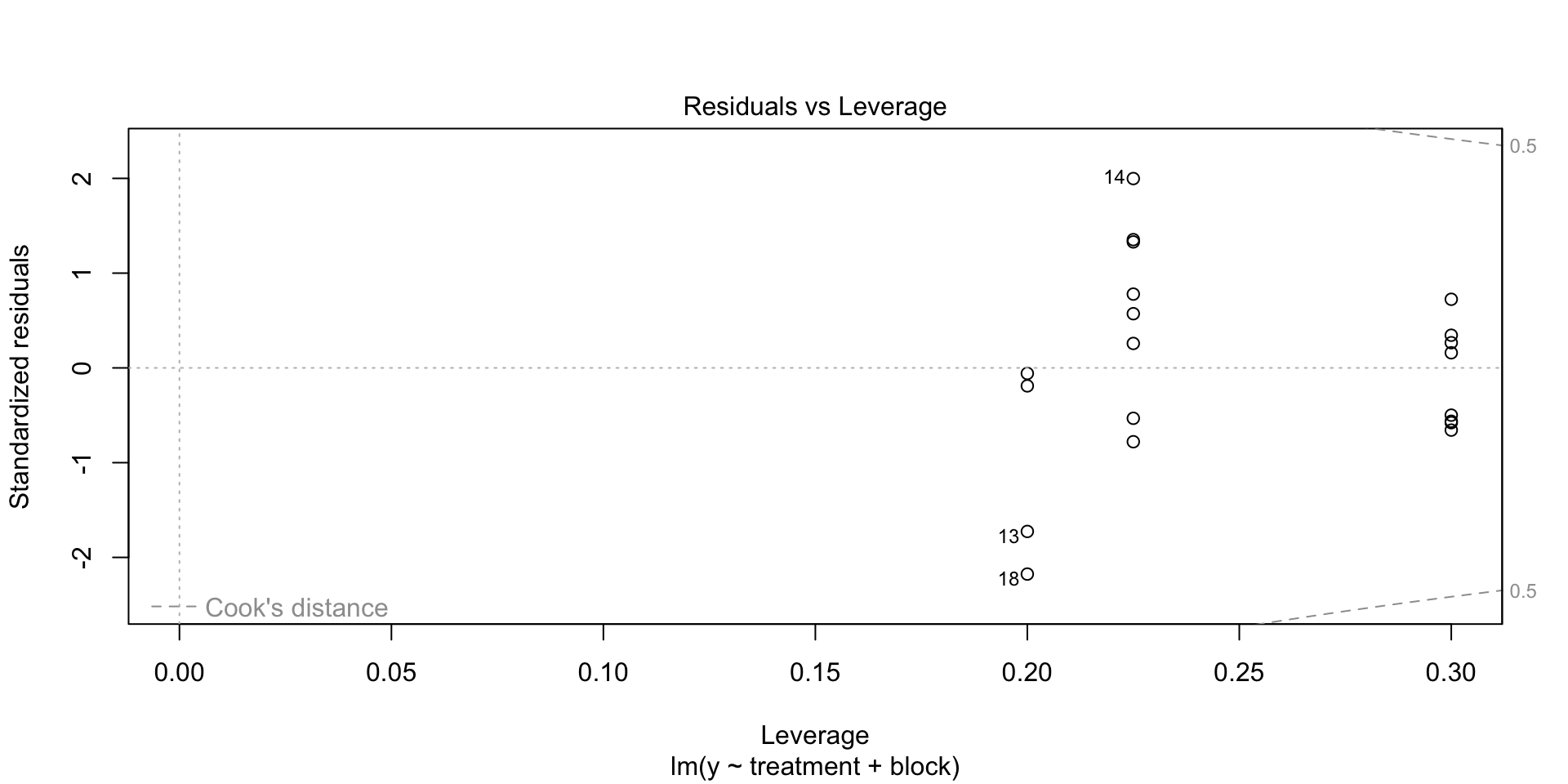
Check the model assumptions using the residual diagnostic plots.
RCBD vs. Two-way ANOVA
Both designs can be analyzed using an additive two-factor model.
| Characteristic | Two-way ANOVA | RCBD |
|---|---|---|
| Factor A | Treatment factor | Treatment factor |
| Factor B | Second treatment factor | Block factor |
| Interaction | Typically included | Not separately estimable |
| Primary interest | Both factors and interaction | Treatment effects |
| Randomization | Across all combinations | Within each block |
Key distinction: In an RCBD, blocks are used to control variability rather than to study a second treatment factor.
Important Considerations
- Every block must contain every treatment.
- Treatments must be randomized within blocks.
- Blocks should account for an important source of variability.
- The model assumes treatment effects are consistent across blocks.
- Blocking is most useful when differences among blocks explain a meaningful amount of variation.
STAT 801A